Chapter 1 Introduction to R

The goal of the first part of this book is to get you up to speed with the basics of R as quickly as possible.

1.1 Installation

Install the latest preview version for getting all features.

Follow the procedures according to your operating system.

Linux: You need to have blas and gfortran installed on your Linux, for installing the coin package.
Rgraphviz requires installation from source("http://bioconductor.org/biocLite.R"), then biocLite("Rgraphviz").
Run the following lines for installing all needed packages (this may take some time):

## listofpackages <- c("arules","arulesViz", "bookdown", "ggplot2", "vioplot", "UsingR", "fpc", "reshape",  "party", "C50", "utils", "rpart", "rpart.plot", "class", "klaR", "e1071", "popbio", "boot", "dplyr", "doParallel", "gbm", "DMwR", "pROC", "neuralnet", "igraph", "RMySQL", "caret", "randomForest", "tm", "wordcloud", "xts", "lubridate", "forecast", "urca", "glmnet", "FSelector", "pls", "emoa", "foreign" )

# newpackages <- listofpackages[!(listofpackages %in% installed.packages()[,"Package"])]
# if(length(newpackages)>0) install.packages(newpackages,dependencies = TRUE)
 
# # install from archive (RPG is no maintained anymore)
# if (!is.element("rgp", installed.packages()[,1]))
# { install.packages("https://cran.r-project.org/src/contrib/Archive/rgp/rgp_0.4-1.tar.gz", 
#                                                     repos = NULL)
# }
## end of installing packages

# in Linux you may need to run several commands (in the terminal) and install additional libraries, e.g. 
# sudo R CMD javareconf
# sudo apt-get install build-essential
# sudo apt-get install libxml2-dev
# sudo apt-get install libpq
# sudo apt-get install libpq-dev
# sudo apt-get install -y libmariadb-client-lgpl-dev
# sudo apt-get install texlive-xetex
# sudo apt-get install r-cran-rmysql

1.2 R and RStudio

R is a programming language for statistical computing and data analysis that supports a variety of programming styles. See R in Wikipedia
R has multiple online resources and books.
R coding style
R-Bloggers
Getting help in R
- RStudio cheat sheet
- Base R cheat sheet
- Advanced R cheat sheet
- Data Visualization cheat sheet
- R Markdown cheatsheet
- [R Markdown Basics] (http://rmarkdown.rstudio.com/authoring_basics.html)
- Python with R and Reticulate Cheatsheet
- caret
- All cheatsheets and translations
- help(" ") command
R as a calculator. Console: It uses the command-line interface.
This document is an RMarkdown document. See bookdown.org

Examples:

x <- c(1,2,3,4,5,6)   # Create ordered collection (vector)
y <- x^2              # Square the elements of x
print(y)              # print (vector) y

## [1]  1  4  9 16 25 36

mean(y)               # Calculate average (arithmetic mean) of (vector) y; result is scalar

## [1] 15.16667

var(y)                # Calculate sample variance

## [1] 178.9667

lm_1 <- lm(y ~ x)     # Fit a linear regression model "y = f(x)" or "y = B0 + (B1 * x)"
                      # store the results as lm_1
print(lm_1)           # Print the model from the (linear model object) lm_1

## 
## Call:
## lm(formula = y ~ x)
## 
## Coefficients:
## (Intercept)            x  
##      -9.333        7.000

summary(lm_1)         # Compute and print statistics for the fit

## 
## Call:
## lm(formula = y ~ x)
## 
## Residuals:
##       1       2       3       4       5       6 
##  3.3333 -0.6667 -2.6667 -2.6667 -0.6667  3.3333 
## 
## Coefficients:
##             Estimate Std. Error t value Pr(>|t|)    
## (Intercept)  -9.3333     2.8441  -3.282 0.030453 *  
## x             7.0000     0.7303   9.585 0.000662 ***
## ---
## Signif. codes:  0 '***' 0.001 '**' 0.01 '*' 0.05 '.' 0.1 ' ' 1
## 
## Residual standard error: 3.055 on 4 degrees of freedom
## Multiple R-squared:  0.9583, Adjusted R-squared:  0.9478 
## F-statistic: 91.88 on 1 and 4 DF,  p-value: 0.000662

                      # of the (linear model object) lm_1
par(mfrow=c(2, 2))    # Request 2x2 plot layout
plot(lm_1)            # Diagnostic plot of regression model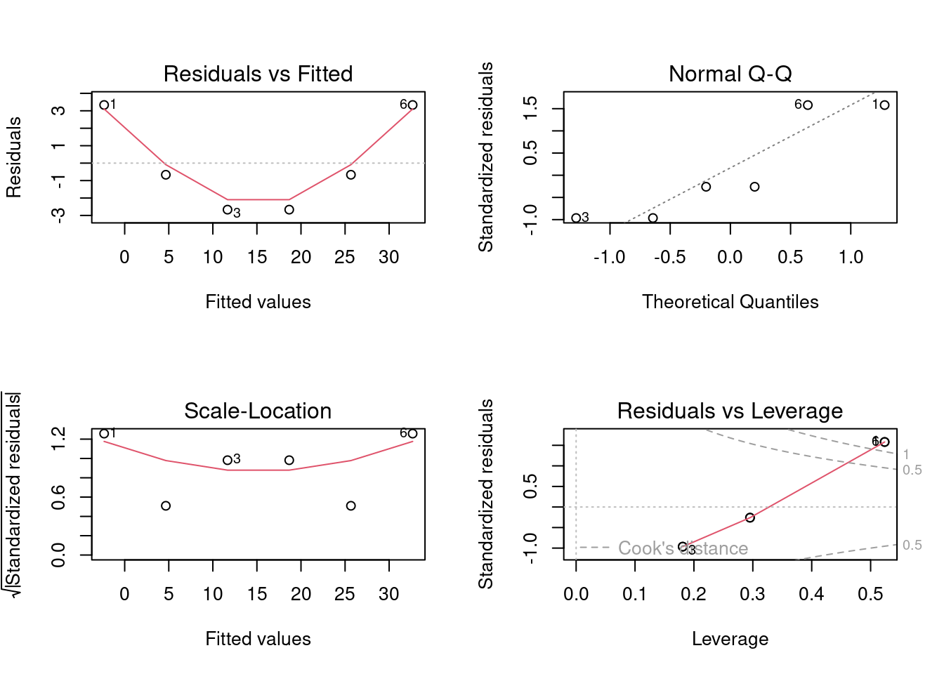

help(lm)
?lm
apropos("lm")

##  [1] ".colMeans"       ".lm.fit"         "colMeans"        "confint.lm"     
##  [5] "contr.helmert"   "dummy.coef.lm"   "glm"             "glm.control"    
##  [9] "glm.fit"         "KalmanForecast"  "KalmanLike"      "KalmanRun"      
## [13] "KalmanSmooth"    "kappa.lm"        "lm"              "lm_1"           
## [17] "lm.fit"          "lm.influence"    "lm.wfit"         "model.matrix.lm"
## [21] "nlm"             "nlminb"          "predict.glm"     "predict.lm"     
## [25] "residuals.glm"   "residuals.lm"    "summary.glm"     "summary.lm"

example(lm)

## 
## lm> require(graphics)
## 
## lm> ## Annette Dobson (1990) "An Introduction to Generalized Linear Models".
## lm> ## Page 9: Plant Weight Data.
## lm> ctl <- c(4.17,5.58,5.18,6.11,4.50,4.61,5.17,4.53,5.33,5.14)
## 
## lm> trt <- c(4.81,4.17,4.41,3.59,5.87,3.83,6.03,4.89,4.32,4.69)
## 
## lm> group <- gl(2, 10, 20, labels = c("Ctl","Trt"))
## 
## lm> weight <- c(ctl, trt)
## 
## lm> lm.D9 <- lm(weight ~ group)
## 
## lm> lm.D90 <- lm(weight ~ group - 1) # omitting intercept
## 
## lm> ## No test: 
## lm> ##D anova(lm.D9)
## lm> ##D summary(lm.D90)
## lm> ## End(No test)
## lm> opar <- par(mfrow = c(2,2), oma = c(0, 0, 1.1, 0))
## 
## lm> plot(lm.D9, las = 1)      # Residuals, Fitted, ...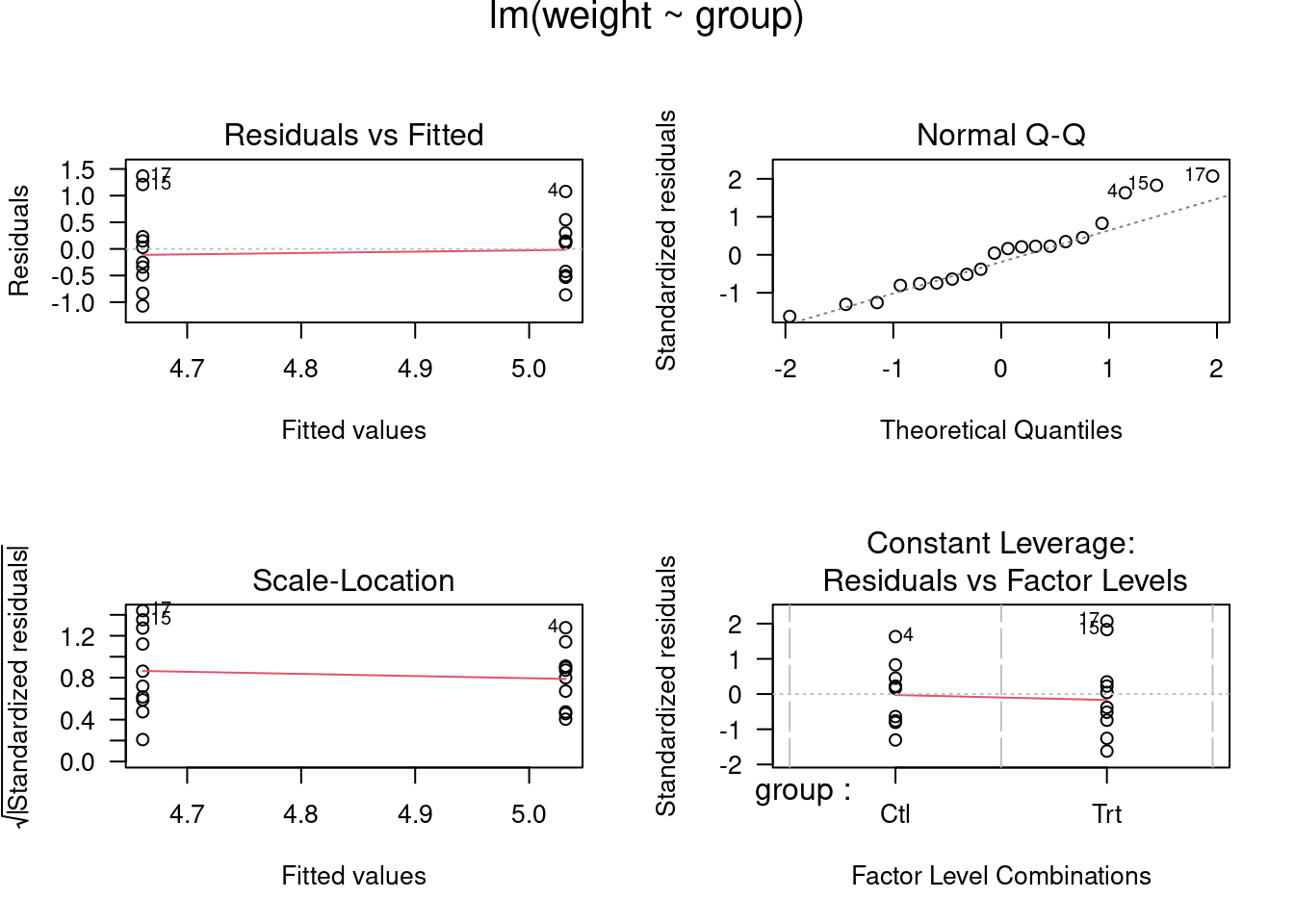

## 
## lm> par(opar)
## 
## lm> ## Don't show: 
## lm> ## model frame :
## lm> stopifnot(identical(lm(weight ~ group, method = "model.frame"),
## lm+                     model.frame(lm.D9)))
## 
## lm> ## End(Don't show)
## lm> ### less simple examples in "See Also" above
## lm> 
## lm> 
## lm>

R script. # A file with R commands # comments source("filewithcommands.R") sink("recordmycommands.lis") savehistory()
From command line:
- Rscript
- Rscript file with -e (e.g. Rscript -e 2+2)
- To exit R: quit()
Variables. R is case sensitive

var1 <- 1:10
vAr1 <- 11:20
var1

##  [1]  1  2  3  4  5  6  7  8  9 10

vAr1

##  [1] 11 12 13 14 15 16 17 18 19 20

Operators
- assign operator <-
- sequence operator, for example: mynums <- 0:20
- arithmetic operators: + - = / ^ %/% (integer division) %% (modulus operator)
The Workspace. Objects.
- ls() objects() ls.str() lists and describes the objects
- rm(x) delete a variable. E.g., rm(totalCost)
- s.str()
- objects()
- str() The structure function provides information about the variable
RStudio, RCommander and RKWard are the well-known IDEs for R (more later).

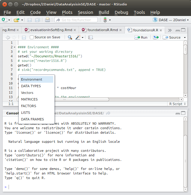
Four # (‘####’) create an environment in RStudio. An environment binds a set of names to a set of values. You can think of an environment as a bag of names.
- Environment basics

Working directories:

# set your working directory
# setwd("~/workingDir/")
getwd()

## [1] "/home/drg/Projects/DASE"

# record R commands:
# sink("recordmycommands.txt", append = TRUE)

1.3 Basic Data Types

class( )
logical: TRUE, FALSE
numeric, integer:
- is.numeric( )
- is.integer( )
character

Examples:

TRUE

## [1] TRUE

class(TRUE)

## [1] "logical"

FALSE

## [1] FALSE

NA  # missing

## [1] NA

class(NA)

## [1] "logical"

## [1] TRUE

## [1] FALSE

NaN

## [1] NaN

class(NaN)

## [1] "numeric"

# numeric data type
2

## [1] 2

class(2)

## [1] "numeric"

2.5

## [1] 2.5

2L  # integer

## [1] 2

class(2L)

## [1] "integer"

is.numeric(2)

## [1] TRUE

is.numeric(2L)

## [1] TRUE

is.integer(2)

## [1] FALSE

is.integer(2L)

## [1] TRUE

is.numeric(NaN)

## [1] TRUE

data type coercion:
- as.numeric( )
- as.character( )
- as.integer( )

Examples:

truenum <- as.numeric(TRUE)
truenum

## [1] 1

class(truenum)

## [1] "numeric"

falsenum <- as.numeric(FALSE)
falsenum

## [1] 0

num2char <- as.character(55)
num2char

## [1] "55"

char2num  <- as.numeric("55.3")

char2int  <- as.integer("55.3")

1.3.1 Mising values

NA stands for Not Available, which is not a number as well. It applies to missing values.
NaN means ‘Not a Number’

Examples:

NA + 1

## [1] NA

mean(c(5,NA,7))

## [1] NA

mean(c(5,NA,7), na.rm=TRUE)  # some functions allow to remove NAs

## [1] 6

1.4 Vectors

Examples:

phases <- c("reqs", "dev", "test1", "test2", "maint")
str(phases)

##  chr [1:5] "reqs" "dev" "test1" "test2" "maint"

is.vector(phases)

## [1] TRUE

thevalues <- c(15, 60, 30, 35, 22)
names(thevalues) <- phases
str(thevalues)

##  Named num [1:5] 15 60 30 35 22
##  - attr(*, "names")= chr [1:5] "reqs" "dev" "test1" "test2" ...

thevalues

##  reqs   dev test1 test2 maint 
##    15    60    30    35    22

A single value is a vector! Example:

aphase <- 44
is.vector(aphase)

## [1] TRUE

length(aphase)

## [1] 1

length(thevalues)

## [1] 5

1.4.1 Coercion for vectors

thevalues1 <- c(15, 60, "30", 35, 22)
class(thevalues1)

## [1] "character"

thevalues1

## [1] "15" "60" "30" "35" "22"

# <-  is equivalent to   assign ( )

assign("costs", c(50, 100, 30))

1.4.2 Vector arithmetic

The operation is carried out in all the elements of the vector. For example:

assign("costs", c(50, 100, 30))
costs/3

## [1] 16.66667 33.33333 10.00000

costs - 5

## [1] 45 95 25

costs <- costs - 5

incomes <- c(200, 800, 10)
earnings <- incomes - costs
sum(earnings)

## [1] 845

# R recycles values in vectors!
vector1 <- c(1,2,3)
vector2 <- c(10,11,12,13,14,15,16)
vector1 + vector2

## Warning in vector1 + vector2: longer object length is not a multiple of shorter
## object length

## [1] 11 13 15 14 16 18 17

Subsetting vectors

### Subsetting vectors  []

phase1 <- phases[1]
phase1

## [1] "reqs"

phase3 <- phases[3]
phase3

## [1] "test1"

thevalues[phase1]

## reqs 
##   15

thevalues["reqs"]

## reqs 
##   15

testphases <- phases[c(3,4)]
thevalues[testphases]

## test1 test2 
##    30    35

### Negative indexes

phases1 <- phases[-5]
phases

## [1] "reqs"  "dev"   "test1" "test2" "maint"

phases1

## [1] "reqs"  "dev"   "test1" "test2"

#phases2 <- phases[-testphases] ## error in argument
phases2 <- phases[-c(3,4)]
phases2

## [1] "reqs"  "dev"   "maint"

### subset using logical vector

phases3 <- phases[c(FALSE, TRUE, TRUE, FALSE)] #recicled first value
phases3

## [1] "dev"   "test1"

selectionv <- c(FALSE, TRUE, TRUE, FALSE)
phases3 <- phases[selectionv]
phases3

## [1] "dev"   "test1"

selectionvec2 <- c(TRUE, FALSE)

thevalues2 <- thevalues[selectionvec2]
thevalues2

##  reqs test1 maint 
##    15    30    22

### Generating regular sequences with  `:` and `seq`

aseqofvalues <- 1:20

aseqofvalues2 <- seq(from=-3, to=3, by=0.5 )
aseqofvalues2

##  [1] -3.0 -2.5 -2.0 -1.5 -1.0 -0.5  0.0  0.5  1.0  1.5  2.0  2.5  3.0

aseqofvalues3 <- seq(0, 100, by=10)
aseqofvalues4 <- aseqofvalues3[c(2, 4, 6, 8)]
aseqofvalues4

## [1] 10 30 50 70

aseqofvalues4 <- aseqofvalues3[-c(2, 4, 6, 8)]
aseqofvalues4

## [1]   0  20  40  60  80  90 100

aseqofvalues3[c(1,2)] <- c(666,888)
aseqofvalues3

##  [1] 666 888  20  30  40  50  60  70  80  90 100

### Logical values in vectors TRUE/FALSE

aseqofvalues3 > 50

##  [1]  TRUE  TRUE FALSE FALSE FALSE FALSE  TRUE  TRUE  TRUE  TRUE  TRUE

aseqofvalues5 <- aseqofvalues3[aseqofvalues3 > 50]
aseqofvalues5

## [1] 666 888  60  70  80  90 100

aseqofvalues6 <- aseqofvalues3[!(aseqofvalues3 > 50)]
aseqofvalues6

## [1] 20 30 40 50

### Comparison functions

aseqofvalues7 <- aseqofvalues3[aseqofvalues3 == 50]
aseqofvalues7

## [1] 50

aseqofvalues8 <- aseqofvalues3[aseqofvalues3 == 22]
aseqofvalues8

## numeric(0)

aseqofvalues9 <- aseqofvalues3[aseqofvalues3 != 50]
aseqofvalues9

##  [1] 666 888  20  30  40  60  70  80  90 100

logicalcond <- aseqofvalues3 >= 50
aseqofvalues10 <- aseqofvalues3[logicalcond]
aseqofvalues10

## [1] 666 888  50  60  70  80  90 100

### Remove Missing Values (NAs)

aseqofvalues3[c(1,2)] <- c(NA,NA)
aseqofvalues3

##  [1]  NA  NA  20  30  40  50  60  70  80  90 100

aseqofvalues3 <- aseqofvalues3[!is.na(aseqofvalues3)]
aseqofvalues3

## [1]  20  30  40  50  60  70  80  90 100

1.5 Arrays and Matrices

Matrices are actually long vectors.

mymat <- matrix(1:12, nrow =2)
mymat

##      [,1] [,2] [,3] [,4] [,5] [,6]
## [1,]    1    3    5    7    9   11
## [2,]    2    4    6    8   10   12

mymat <- matrix(1:12, ncol =3)
mymat

##      [,1] [,2] [,3]
## [1,]    1    5    9
## [2,]    2    6   10
## [3,]    3    7   11
## [4,]    4    8   12

mymat <- matrix(1:12, nrow=2, byrow = TRUE)
mymat

##      [,1] [,2] [,3] [,4] [,5] [,6]
## [1,]    1    2    3    4    5    6
## [2,]    7    8    9   10   11   12

mymat <- matrix(1:12, nrow=3, ncol=4)
mymat

##      [,1] [,2] [,3] [,4]
## [1,]    1    4    7   10
## [2,]    2    5    8   11
## [3,]    3    6    9   12

mymat <- matrix(1:12, nrow=3, ncol=4, byrow=TRUE)
mymat

##      [,1] [,2] [,3] [,4]
## [1,]    1    2    3    4
## [2,]    5    6    7    8
## [3,]    9   10   11   12

### recycling
mymat <- matrix(1:5, nrow=3, ncol=4, byrow=TRUE)

## Warning in matrix(1:5, nrow = 3, ncol = 4, byrow = TRUE): data length [5] is not
## a sub-multiple or multiple of the number of rows [3]

mymat

##      [,1] [,2] [,3] [,4]
## [1,]    1    2    3    4
## [2,]    5    1    2    3
## [3,]    4    5    1    2

### rbind  cbind

cbind(1:3, 1:3)

##      [,1] [,2]
## [1,]    1    1
## [2,]    2    2
## [3,]    3    3

rbind(1:3, 1:3)

##      [,1] [,2] [,3]
## [1,]    1    2    3
## [2,]    1    2    3

mymat <- matrix(1)

mymat <- matrix(1:8, nrow=2, ncol=4, byrow=TRUE)
mymat

##      [,1] [,2] [,3] [,4]
## [1,]    1    2    3    4
## [2,]    5    6    7    8

rbind(mymat, 9:12)

##      [,1] [,2] [,3] [,4]
## [1,]    1    2    3    4
## [2,]    5    6    7    8
## [3,]    9   10   11   12

mymat <- cbind(mymat, c(5,9))
mymat

##      [,1] [,2] [,3] [,4] [,5]
## [1,]    1    2    3    4    5
## [2,]    5    6    7    8    9

mymat  <- matrix(1:8, byrow = TRUE, nrow=2)
mymat

##      [,1] [,2] [,3] [,4]
## [1,]    1    2    3    4
## [2,]    5    6    7    8

rownames(mymat) <- c("row1", "row2")
mymat

##      [,1] [,2] [,3] [,4]
## row1    1    2    3    4
## row2    5    6    7    8

colnames(mymat) <- c("col1", "col2", "col3", "col4")
mymat

##      col1 col2 col3 col4
## row1    1    2    3    4
## row2    5    6    7    8

mymat2 <- matrix(1:12, byrow=TRUE, nrow=3, dimnames=list(c("row1", "row2", "row3"),
                                                         c("col1", "col2", "col3", "col4")))
mymat2

##      col1 col2 col3 col4
## row1    1    2    3    4
## row2    5    6    7    8
## row3    9   10   11   12

### Coercion in Arrays

matnum <- matrix(1:8, ncol = 2)
matnum

##      [,1] [,2]
## [1,]    1    5
## [2,]    2    6
## [3,]    3    7
## [4,]    4    8

matchar <- matrix(LETTERS[1:6], nrow = 4, ncol = 3)
matchar

##      [,1] [,2] [,3]
## [1,] "A"  "E"  "C" 
## [2,] "B"  "F"  "D" 
## [3,] "C"  "A"  "E" 
## [4,] "D"  "B"  "F"

matchars <- cbind(matnum, matchar)
matchars

##      [,1] [,2] [,3] [,4] [,5]
## [1,] "1"  "5"  "A"  "E"  "C" 
## [2,] "2"  "6"  "B"  "F"  "D" 
## [3,] "3"  "7"  "C"  "A"  "E" 
## [4,] "4"  "8"  "D"  "B"  "F"

### Subsetting  

mymat3 <- matrix(sample(-8:15, 12), nrow=3)  #sample 12 numbers between -8 and 15
mymat3

##      [,1] [,2] [,3] [,4]
## [1,]    0    5   -3   -2
## [2,]    2    7    3   13
## [3,]   -1    1    9   11

mymat3[2,3]

## [1] 3

mymat3[1,4]

## [1] -2

mymat3[3,]

## [1] -1  1  9 11

mymat3[,4]

## [1] -2 13 11

mymat3[5] # counts elements by column

## [1] 7

mymat3[9]

## [1] 9

## Subsetting multiple elements

mymat3[2, c(1,3)]

## [1] 2 3

mymat3[c(2,3), c(1,3,4)]

##      [,1] [,2] [,3]
## [1,]    2    3   13
## [2,]   -1    9   11

rownames(mymat3) <- c("r1", "r2", "r3")
colnames(mymat3) <- c("c1", "c2", "c3", "c4")
mymat3["r2", c("c1", "c3")]

## c1 c3 
##  2  3

### Subset by logical vector
mymat3[c(FALSE, TRUE, FALSE),
       c(TRUE, FALSE, TRUE, FALSE)]

## c1 c3 
##  2  3

mymat3[c(FALSE, TRUE, TRUE),
       c(TRUE, FALSE, TRUE, TRUE)]

##    c1 c3 c4
## r2  2  3 13
## r3 -1  9 11

### matrix arithmetic

row1 <- c(220, 137)
row2 <- c(345, 987)
row3 <- c(111, 777)

mymat4 <- rbind(row1, row2, row3)
rownames(mymat4) <- c("row_1", "row_2", "row_3")
colnames(mymat4) <- c("col_1", "col_2")
mymat4

##       col_1 col_2
## row_1   220   137
## row_2   345   987
## row_3   111   777

mymat4/10

##       col_1 col_2
## row_1  22.0  13.7
## row_2  34.5  98.7
## row_3  11.1  77.7

mymat4 -100

##       col_1 col_2
## row_1   120    37
## row_2   245   887
## row_3    11   677

mymat5 <- rbind(c(50,50), c(10,10), c(100,100))
mymat5

##      [,1] [,2]
## [1,]   50   50
## [2,]   10   10
## [3,]  100  100

mymat4 - mymat5

##       col_1 col_2
## row_1   170    87
## row_2   335   977
## row_3    11   677

mymat4 * (mymat5/100)

##       col_1 col_2
## row_1 110.0  68.5
## row_2  34.5  98.7
## row_3 111.0 777.0

### index matrices

m1 <- array(1:20, dim=c(4,5))
m1

##      [,1] [,2] [,3] [,4] [,5]
## [1,]    1    5    9   13   17
## [2,]    2    6   10   14   18
## [3,]    3    7   11   15   19
## [4,]    4    8   12   16   20

index <- array(c(1:3, 3:1), dim=c(3,2))
index

##      [,1] [,2]
## [1,]    1    3
## [2,]    2    2
## [3,]    3    1

#use the "index matrix" as the index for the other matrix
m1[index] <-0
m1

##      [,1] [,2] [,3] [,4] [,5]
## [1,]    1    5    0   13   17
## [2,]    2    0   10   14   18
## [3,]    0    7   11   15   19
## [4,]    4    8   12   16   20

1.6 Factors

Factors are variables in R which take on a limited number of different values; such variables are often referred to as ‘categorical variables’ and ‘enumerated type’.
Factors in R are stored as a vector of integer values with a corresponding set of character values to use when the factor is displayed.
The function factor is used to encode a vector as a factor

personnel <- c("Analyst1", "ManagerL2", "Analyst1", "Analyst2",
               "Boss", "ManagerL1", "ManagerL2", "Programmer1",
               "Programmer2", "Programmer3", "Designer1","Designer2",
               "OtherStaff")  # staff in a company

personnel_factors <- factor(personnel)
personnel_factors  #sorted alphabetically

##  [1] Analyst1    ManagerL2   Analyst1    Analyst2    Boss        ManagerL1  
##  [7] ManagerL2   Programmer1 Programmer2 Programmer3 Designer1   Designer2  
## [13] OtherStaff 
## 11 Levels: Analyst1 Analyst2 Boss Designer1 Designer2 ManagerL1 ... Programmer3

str(personnel_factors)

##  Factor w/ 11 levels "Analyst1","Analyst2",..: 1 7 1 2 3 6 7 9 10 11 ...

personnel2 <- factor(personnel, 
                     levels = c("Boss", "ManagerL1", "ManagerL2", 
                                "Analyst1", "Analyst2",  "Designer1",
                                "Designer2", "Programmer1", "Programmer2", 
                                "Programmer3", "OtherStaff")) 
                                #do not duplicate the same factors
personnel2

##  [1] Analyst1    ManagerL2   Analyst1    Analyst2    Boss        ManagerL1  
##  [7] ManagerL2   Programmer1 Programmer2 Programmer3 Designer1   Designer2  
## [13] OtherStaff 
## 11 Levels: Boss ManagerL1 ManagerL2 Analyst1 Analyst2 Designer1 ... OtherStaff

str(personnel2)

##  Factor w/ 11 levels "Boss","ManagerL1",..: 4 3 4 5 1 2 3 8 9 10 ...

# a factor's levels will always be character values.

levels(personnel2) <- c("B", "M1", "M2", "A1", "A2",
                        "D1", "D2", "P1", "P2", "P3", "OS")
personnel2

##  [1] A1 M2 A1 A2 B  M1 M2 P1 P2 P3 D1 D2 OS
## Levels: B M1 M2 A1 A2 D1 D2 P1 P2 P3 OS

personnel3 <- factor(personnel,
                     levels = c("Boss", "ManagerL1", "ManagerL2",
                                "Analyst1", "Analyst2",  "Designer1",
                                "Designer2", "Programmer1", "Programmer2",
                                "Programmer3", "OtherStaff"),
                     c("B", "M1", "M2", "A1", "A2", "D1", "D2",
                       "P1", "P2", "P3", "OS"))
personnel3

##  [1] A1 M2 A1 A2 B  M1 M2 P1 P2 P3 D1 D2 OS
## Levels: B M1 M2 A1 A2 D1 D2 P1 P2 P3 OS

### Nominal versus ordinal, ordered factors
personnel3[1] < personnel3[2]  # error, factors not ordered

## Warning in Ops.factor(personnel3[1], personnel3[2]): '<' not meaningful for
## factors

## [1] NA

tshirts <- c("M", "L", "S", "S", "L", "M", "L", "M")

tshirt_factor <- factor(tshirts, ordered = TRUE,
                        levels = c("S", "M", "L"))
tshirt_factor

## [1] M L S S L M L M
## Levels: S < M < L

tshirt_factor[1] < tshirt_factor[2]

## [1] TRUE

1.7 Lists

Lists are the R objects which contain elements of different types: numbers, strings, vectors and other lists. A list can also contain a matrix or a function as one of their elements. A list is created using list() function.

Operators for subsetting lists include: - ‘[’ returns a list - ’[[’ returns the list element - ‘$’ returns the content of that element in the list]<-1

cbo <- jdt$cbo bugs <- jdt$bugs