1 Introduction to R

The goal of the first part of this book is to get you up to speed with the basics of R as quickly as possible.

1.1 Installation

Install the latest preview version for getting all features.

Follow the procedures according to your operating system.

Linux: You need to have blas and gfortran installed on your Linux, for installing the coin package.
Rgraphviz requires Bioconductor: BiocManager::install("Rgraphviz") (install BiocManager from CRAN first if needed).
Run the following lines for installing all needed packages (this may take some time):

## listofpackages <- c("arules","arulesViz", "quarto", "ggplot2", "vioplot", "UsingR", "fpc", "reshape", "partykit", "C50", "utils", "rpart", "rpart.plot", "class", "klaR", "e1071", "popbio", "boot", "dplyr", "doParallel", "gbm", "themis", "pROC", "neuralnet", "igraph", "RMariaDB", "tidymodels", "ranger", "tm", "wordcloud", "xts", "lubridate", "forecast", "urca", "glmnet", "FSelectorRcpp", "pls", "emoa", "foreign" )

# newpackages <- listofpackages[!(listofpackages %in% installed.packages()[,"Package"])]
# if(length(newpackages)>0) install.packages(newpackages,dependencies = TRUE)
 
# # install from archive (RPG is no maintained anymore)
# if (!is.element("rgp", installed.packages()[,1]))
# { install.packages("https://cran.r-project.org/src/contrib/Archive/rgp/rgp_0.4-1.tar.gz", 
#                                                     repos = NULL)
# }
## end of installing packages

# in Linux you may need to run several commands (in the terminal) and install additional libraries, e.g. 
# sudo R CMD javareconf
# sudo apt-get install build-essential
# sudo apt-get install libxml2-dev
# sudo apt-get install libpq
# sudo apt-get install libpq-dev
# sudo apt-get install -y libmariadb-client-lgpl-dev
# sudo apt-get install texlive-xetex
# sudo apt-get install r-cran-rmysql

1.2 R and RStudio

R is a programming language for statistical computing and data analysis that supports a variety of programming styles. See R in Wikipedia
R has multiple online resources and books.
R coding style
R-Bloggers
Getting help in R
R as a calculator. Console: It uses the command-line interface.
This document is an RMarkdown document. See bookdown.org

Examples:

loc <- c(120, 240, 310, 480, 560, 700)   # Lines of code per module
defects <- c(0, 1, 1, 2, 3, 4)           # Observed post-release defects
print(defects)                            # Print vector
mean(defects)                             # Average defects per module
var(defects)                              # Variability of defects
lm_1 <- lm(defects ~ loc)                 # Simple defect-risk trend model
print(lm_1)
summary(lm_1)
par(mfrow=c(2, 2))    # Request 2x2 plot layout
plot(lm_1)            # Diagnostic plots for the fitted model

help(lm)
?lm
apropos("lm")
example(lm)

R script. # A file with R commands # comments source("filewithcommands.R") sink("recordmycommands.lis") savehistory()
From command line:
- Rscript
- Rscript file with -e (e.g. Rscript -e 2+2)
- To exit R: quit()
Variables. R is case sensitive

var1 <- c("Auth", "Billing", "Search")
vAr1 <- c("auth", "billing", "search")
var1
vAr1

Operators
- assign operator <-
- sequence operator, for example: mynums <- 0:20
- arithmetic operators: + - = / ^ %/% (integer division) %% (modulus operator)
The Workspace. Objects.
- ls() objects() ls.str() lists and describes the objects
- rm(x) delete a variable. E.g., rm(totalCost)
- s.str()
- objects()
- str() The structure function provides information about the variable
RStudio, RCommander and RKWard are the well-known IDEs for R (more later).

Four # (‘####’) create an environment in RStudio. An environment binds a set of names to a set of values. You can think of an environment as a bag of names.
- Environment basics

Working directories:

# set your working directory
# setwd("~/workingDir/")
getwd()
# record R commands:
# sink("recordmycommands.txt", append = TRUE)

1.3 Basic Data Types

class( )
logical: TRUE, FALSE
numeric, integer:
- is.numeric( )
- is.integer( )
character

Examples:

TRUE
class(TRUE)
FALSE
NA  # missing
class(NA)
T
F
NaN
class(NaN)

# numeric data type
2
class(2)
2.5
2L  # integer
class(2L)

is.numeric(2)
is.numeric(2L)
is.integer(2)
is.integer(2L)
is.numeric(NaN)

data type coercion:
- as.numeric( )
- as.character( )
- as.integer( )

Examples:

truenum <- as.numeric(TRUE)
truenum
class(truenum)
falsenum <- as.numeric(FALSE)
falsenum

num2char <- as.character(55)
num2char
char2num  <- as.numeric("55.3")

char2int  <- as.integer("55.3")

1.3.1 Missing values

NA stands for Not Available, which is not a number as well. It applies to missing values.
NaN means ‘Not a Number’

Examples:

NA + 1
mean(c(5,NA,7))
mean(c(5,NA,7), na.rm=TRUE)  # some functions allow to remove NAs

1.4 Vectors

Examples:

phases <- c("reqs", "dev", "test1", "test2", "maint")
str(phases)
is.vector(phases)

thevalues <- c(15, 60, 30, 35, 22)
names(thevalues) <- phases
str(thevalues)
thevalues

A single value is a vector! Example:

aphase <- 44
is.vector(aphase)

length(aphase)
length(thevalues)

1.4.1 Coercion for vectors

thevalues1 <- c(15, 60, "30", 35, 22)
class(thevalues1)
thevalues1


# <-  is equivalent to   assign ( )

assign("costs", c(50, 100, 30))

1.4.2 Vector arithmetic

The operation is carried out in all the elements of the vector. For example:

assign("costs", c(50, 100, 30))
costs/3
costs - 5
costs <- costs - 5

incomes <- c(200, 800, 10)
earnings <- incomes - costs
sum(earnings)

# R recycles values in vectors!
vector1 <- c(1,2,3)
vector2 <- c(10,11,12,13,14,15,16)
vector1 + vector2

Subsetting vectors

### Subsetting vectors  []

phase1 <- phases[1]
phase1
phase3 <- phases[3]
phase3

thevalues[phase1]
thevalues["reqs"]

testphases <- phases[c(3,4)]
thevalues[testphases]

### Negative indexes

phases1 <- phases[-5]
phases
phases1

#phases2 <- phases[-testphases] ## error in argument
phases2 <- phases[-c(3,4)]
phases2

### subset using logical vector

phases3 <- phases[c(FALSE, TRUE, TRUE, FALSE)] #recicled first value
phases3

selectionv <- c(FALSE, TRUE, TRUE, FALSE)
phases3 <- phases[selectionv]
phases3

selectionvec2 <- c(TRUE, FALSE)

thevalues2 <- thevalues[selectionvec2]
thevalues2


### Generating regular sequences with  `:` and `seq`

aseqofvalues <- 1:20

aseqofvalues2 <- seq(from=-3, to=3, by=0.5 )
aseqofvalues2

aseqofvalues3 <- seq(0, 100, by=10)
aseqofvalues4 <- aseqofvalues3[c(2, 4, 6, 8)]
aseqofvalues4
aseqofvalues4 <- aseqofvalues3[-c(2, 4, 6, 8)]
aseqofvalues4

aseqofvalues3[c(1,2)] <- c(666,888)
aseqofvalues3

### Logical values in vectors TRUE/FALSE

aseqofvalues3 > 50
aseqofvalues5 <- aseqofvalues3[aseqofvalues3 > 50]
aseqofvalues5
aseqofvalues6 <- aseqofvalues3[!(aseqofvalues3 > 50)]
aseqofvalues6

### Comparison functions

aseqofvalues7 <- aseqofvalues3[aseqofvalues3 == 50]
aseqofvalues7

aseqofvalues8 <- aseqofvalues3[aseqofvalues3 == 22]
aseqofvalues8

aseqofvalues9 <- aseqofvalues3[aseqofvalues3 != 50]
aseqofvalues9

logicalcond <- aseqofvalues3 >= 50
aseqofvalues10 <- aseqofvalues3[logicalcond]
aseqofvalues10


### Remove Missing Values (NAs)

aseqofvalues3[c(1,2)] <- c(NA,NA)
aseqofvalues3

aseqofvalues3 <- aseqofvalues3[!is.na(aseqofvalues3)]
aseqofvalues3

1.5 Arrays and Matrices

Matrices are actually long vectors.

mymat <- matrix(1:12, nrow =2)
mymat

mymat <- matrix(1:12, ncol =3)
mymat

mymat <- matrix(1:12, nrow=2, byrow = TRUE)
mymat

mymat <- matrix(1:12, nrow=3, ncol=4)
mymat

mymat <- matrix(1:12, nrow=3, ncol=4, byrow=TRUE)
mymat

### recycling
mymat <- matrix(1:5, nrow=3, ncol=4, byrow=TRUE)
mymat

### rbind  cbind

cbind(1:3, 1:3)
rbind(1:3, 1:3)

mymat <- matrix(1)

mymat <- matrix(1:8, nrow=2, ncol=4, byrow=TRUE)
mymat

rbind(mymat, 9:12)
mymat <- cbind(mymat, c(5,9))
mymat

mymat  <- matrix(1:8, byrow = TRUE, nrow=2)
mymat
rownames(mymat) <- c("row1", "row2")
mymat
colnames(mymat) <- c("col1", "col2", "col3", "col4")
mymat

mymat2 <- matrix(1:12, byrow=TRUE, nrow=3, dimnames=list(c("row1", "row2", "row3"),
                                                         c("col1", "col2", "col3", "col4")))
mymat2

### Coercion in Arrays

matnum <- matrix(1:8, ncol = 2)
matnum
matchar <- matrix(LETTERS[1:6], nrow = 4, ncol = 3)
matchar

matchars <- cbind(matnum, matchar)
matchars

### Subsetting  

mymat3 <- matrix(sample(-8:15, 12), nrow=3)  #sample 12 numbers between -8 and 15
mymat3
mymat3[2,3]
mymat3[1,4]
mymat3[3,]
mymat3[,4]
mymat3[5] # counts elements by column
mymat3[9]

## Subsetting multiple elements

mymat3[2, c(1,3)]
mymat3[c(2,3), c(1,3,4)]

rownames(mymat3) <- c("r1", "r2", "r3")
colnames(mymat3) <- c("c1", "c2", "c3", "c4")
mymat3["r2", c("c1", "c3")]

### Subset by logical vector
mymat3[c(FALSE, TRUE, FALSE),
       c(TRUE, FALSE, TRUE, FALSE)]
mymat3[c(FALSE, TRUE, TRUE),
       c(TRUE, FALSE, TRUE, TRUE)]

### matrix arithmetic

row1 <- c(220, 137)
row2 <- c(345, 987)
row3 <- c(111, 777)

mymat4 <- rbind(row1, row2, row3)
rownames(mymat4) <- c("row_1", "row_2", "row_3")
colnames(mymat4) <- c("col_1", "col_2")
mymat4

mymat4/10
mymat4 -100

mymat5 <- rbind(c(50,50), c(10,10), c(100,100))
mymat5

mymat4 - mymat5

mymat4 * (mymat5/100)


### index matrices

m1 <- array(1:20, dim=c(4,5))
m1

index <- array(c(1:3, 3:1), dim=c(3,2))
index

#use the "index matrix" as the index for the other matrix
m1[index] <-0
m1

1.6 Factors

Factors are variables in R which take on a limited number of different values; such variables are often referred to as ‘categorical variables’ and ‘enumerated type’.
Factors in R are stored as a vector of integer values with a corresponding set of character values to use when the factor is displayed.
The function factor is used to encode a vector as a factor

personnel <- c("Analyst1", "ManagerL2", "Analyst1", "Analyst2",
               "Boss", "ManagerL1", "ManagerL2", "Programmer1",
               "Programmer2", "Programmer3", "Designer1","Designer2",
               "OtherStaff")  # staff in a company

personnel_factors <- factor(personnel)
personnel_factors  #sorted alphabetically
str(personnel_factors)

personnel2 <- factor(personnel, 
                     levels = c("Boss", "ManagerL1", "ManagerL2", 
                                "Analyst1", "Analyst2",  "Designer1",
                                "Designer2", "Programmer1", "Programmer2", 
                                "Programmer3", "OtherStaff")) 
                                #do not duplicate the same factors
personnel2
str(personnel2)

# a factor's levels will always be character values.

levels(personnel2) <- c("B", "M1", "M2", "A1", "A2",
                        "D1", "D2", "P1", "P2", "P3", "OS")
personnel2

personnel3 <- factor(personnel,
                     levels = c("Boss", "ManagerL1", "ManagerL2",
                                "Analyst1", "Analyst2",  "Designer1",
                                "Designer2", "Programmer1", "Programmer2",
                                "Programmer3", "OtherStaff"),
                     c("B", "M1", "M2", "A1", "A2", "D1", "D2",
                       "P1", "P2", "P3", "OS"))
personnel3


### Nominal versus ordinal, ordered factors
personnel3[1] < personnel3[2]  # error, factors not ordered

tshirts <- c("M", "L", "S", "S", "L", "M", "L", "M")

tshirt_factor <- factor(tshirts, ordered = TRUE,
                        levels = c("S", "M", "L"))
tshirt_factor

tshirt_factor[1] < tshirt_factor[2]

1.7 Lists

Lists are the R objects which contain elements of different types: numbers, strings, vectors and other lists. A list can also contain a matrix or a function as one of their elements. A list is created using list() function.

Operators for subsetting lists include: - ‘[’ returns a list - ‘[[’ returns the list element - ‘$’ returns the content of that element in the list

c("R good times", 190, 5)

song <- list("R good times", 190, 5)
is.list(song)
str(song)

names(song) <- c("title", "duration", "track")
song
song$title

song2 <- list(title="Good Friends", 
              duration = 125,
              track = 2,
              rank = 6)

song3 <- list(title="Many Friends", 
              duration = 125,
              track= 2,
              rank = 1,
              similar2 = song2)

song[1]
song$title
str(song[1])
song[[1]]
str(song[[1]])

song2[3]

song3[5]  # a list
str(song3[5])
song3[[5]]
song3$similar2

song[c(1,3)]
str(song[c(1,3)])

result <- song[c(1,3)]
result[1]
result[[1]]
str(result)
result$title
result$track

# access with [[ to content 
song3[[5]][[1]]
song3$similar2[[1]]

# Subsets
### subset by names
song[c("title", "track")]

song3["similar2"]
resultsimilar <- song3["similar2"]
str(resultsimilar)
resultsimilar1 <-song3[["similar2"]]
str(resultsimilar1)
resultsimilar1$title

# subset by logicals
song[c(TRUE, FALSE, TRUE, FALSE)]
result3 <- song[c(TRUE, FALSE, TRUE, FALSE)]  # is a list of two elements

# extending the list
shared <- c("Hillary", "Mari", "Mikel", "Patty")

song3$shared <- shared
str(song3)

cities <- list("Bilbao", "New York", "Tartu")
song3[["cities"]] <- cities
str(song3)

1.8 Data frames

A data frame is the data structure most often used for data analyses. A data frame is a list of equal-length vectors. Each element of the list can be thought of as a column and the length of each element of the list is the number of rows. As a result, data frames can store different classes of objects in each column (i.e. numeric, character, factor).

The tidyverse package provides a version of the data frame called tibble

thenames <- c("Ane", "Mike", "Laura", "Viktoria", "Martin")
ages <- c(44, 20, 33, 15, 65)
employee <- c(FALSE, FALSE, TRUE, TRUE, FALSE)

mydataframe <- data.frame(thenames, ages, employee)
mydataframe

names(mydataframe) <- c("FirstName", "Age", "Employee")
str(mydataframe)

#strings are not factors!

mydataframe <- data.frame(thenames, ages, employee,
                          stringsAsFactors=FALSE)
names(mydataframe) <- c("FirstName", "Age", "Employee")
str(mydataframe)


# subset data frame

mydataframe[4,2]
mydataframe[4, "Age"]
mydataframe[, "FirstName"]

mydataframe[c(2,5), c("Age", "Employee")]
matfromframe <- as.matrix(mydataframe[c(2,5), c("Age", "Employee")])
str(matfromframe)

mydataframe[3]

# convert to vector
mydf0 <- mydataframe[3] #data.frame
str(mydf0)


myvec <- mydataframe[[3]]  #vector
str(myvec)

mydf0asvec <- as.vector(mydataframe[3]) # but it doesn't work . Use [[]]
str(mydf0asvec)
mydf0asvec <- as.vector(mydataframe[[3]])
str(mydf0asvec)

# add column
height <- c(166, 165, 158, 176, 199)
weight <- c(66, 77, 99, 88, 109)
mydataframe$height <- height 
mydataframe[["weight"]] <- weight
mydataframe

# add a column 

birthplace <- c("Tallinn", "London", "Donostia", "Paris", "New York")

mydataframe <- cbind(mydataframe, birthplace)
mydataframe

# add a row 

anton <- data.frame(FirstName = "Anton", Age = 77, Employee=TRUE, height= 170, weight = 65, birthplace ="Amsterdam", stringsAsFactors=FALSE)
mydataframe <- rbind (mydataframe, anton)
mydataframe

# sorting 

mydataframeSorted <- mydataframe[order(mydataframe$Age, decreasing = TRUE), ]  #all columns
mydataframeSorted
mydataframeSorted2 <- mydataframe[order(mydataframe$Age, decreasing = TRUE), c(1,2,6) ]
mydataframeSorted2

1.9 R Functional Functions

R is a functional language and there are some special functions provided: apply(), lapply(), sapply(), tapply(), mapply(), vapply()

One of its main strengths lies in the use of the functions apply() (and all its variations) on lists, matrices, data frames or other data structures. The tidyverse package provides the purrr package for functional programming. The topic of functional programming lies beyond the purpose of this introduction.

Most of the commands that we use in our scripts are functions applied to data.

1.10 Environments

An environment is a place where R stores variables that is where R binds a set of names to a set of object values. An environment is something like a bag or a list of names. Every name in an environment is unique.

The top level environment R_GlobalEnv is created when we start up R and is the global environment. Every environment has parent environment. When we define a function, a new environment is created.

1.10.1 Global variables, local variables and programming scope

Global variables are those variables which exists throughout the execution of a program. Local variables are those variables which exist only within a certain part of a program like a function. The super-assignment operator, <<-, is used to make assignments to global variables or to make assignments in the parent environment.

# variables and functions in the current environment
ls()
# to get the current environment
environment()
# the base environment is the environment of the base package
baseenv()

# list of environments
search()

# functions and environments 
# in this example we do not return any value 

myfunction <- function() {
  myvar_a<- 50
  myfunctioninside <- function() {
  myvar_a <- 100
  # myvar_a <<- 100
  print(myvar_a)
  }
  myfunctioninside()
  print(myvar_a)
  # myvar_a <<- 100
}

myvar_a <- 10
myfunction()
print(myvar_a)

# create environment
my_env <- new.env()
my_env

ls(my_env)
character(0)
assign("myvar_a", 700, envir=my_env)
my_env$mytext = " a text"
ls(my_env)

myvar_a
my_env$myvar_a

parent.env(my_env)
get('myvar_a', envir=my_env)

1.11 Reading Data

R is capable of reading most formats including CSV, MS Excel formats (xlsx, etc.) as well as other statistical packages (e.g. SAS, SPSS, etc.) and data mining tools such as ARFF (Weka’s format).

R also provides has two native data formats, Rdata and Rds. These formats are used when leaving or starting an R session so that R objects can be stored or retrieved to continue in the same state). While Rdata is used to save multiple R objects, Rds is used to save a single R object.

load("data.rdata") # It is needed to be in the same directory (setwd())

To read CSV (Comma Separated Values) files in R

# Import the data and look at the first six rows
f <- read.csv("data.csv")
head(f)

To read ARFF files, we can use the foreign library.

library(foreign)
isbsg <- read.arff("datasets/effortEstimation/isbsg10teaser.arff")

mydataISBSG <- isbsg[, c("FS", "N_effort")]
str(mydataISBSG)

1.12 Plots

There are several graphic packages that are recommended, in particular ggplot. However, there is some basic support in the R base for graphics. The following Figure @ref(fig:plotExample) shows a simple plot.

plot(mydataISBSG$FS, mydataISBSG$N_effort)

1.13 Control flow in R

R provides most common control flow structures found in most languages

if

x <- 6
if (x >= 5) {
    "x is greater than or equals 5"
} else {
    "x is smaller than 5"
}

ifelse

kc1 <- read.csv("datasets/defectPred/unified/Unified-file.csv", stringsAsFactors = FALSE)
kc1 <- kc1[, c("McCC", "CLOC", "PDA", "PUA", "LLOC", "LOC", "bug")]
kc1$Defective <- ifelse(kc1$bug > 0, "Y", "N")
kc1$bug <- NULL
kc1$Defective <- ifelse(kc1$Defective == "Y", 1, 0)
head(kc1, 1)

for loops

for(x in 1:5){
  print(x)
}

1.14 Built-in Datasets

R comes with some built-in datasets ready to use Description of datasets http://www.sthda.com/english/wiki/r-built-in-data-sets

data()  #list of datasets already available

Then, to load a dataset is as follows.

# load the mtcars  Motor Trend Car Road Tests
data("mtcars")

And another example.

# Monthly Airline Passenger Numbers 1949-1960
# Time series object ts() convert a vector to a time series
data("AirPassengers")
str(AirPassengers)
plot(AirPassengers)

1.15 Other tools with R

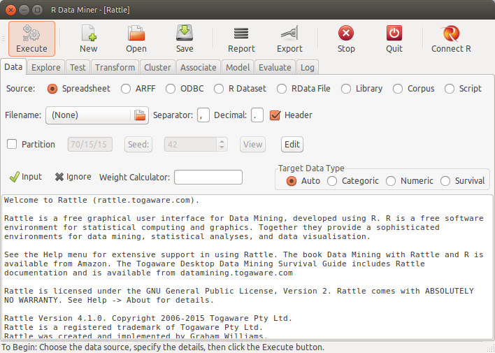
1.15.1 Rattle

There is graphical interface, Rattle, that allow us to perform some data mining tasks with R (Williams 2011).

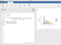
1.15.2 Jamovi

GUI for statistical analysis in R. It allow us to export the actual R code. Its Website is: https://www.jamovi.org/

1.15.3 JASP

There is another GUI for statistics, JASP, but it is not so easy at the moment to export the R code. https://jasp-stats.org/