26  Social Network Analysis in SE

In this example, we will data from the MSR14 challenge. Further information and datasets: http://openscience.us/repo/msr/msr14.html

Similar databases can be obtained using MetricsGrimoire or other tools.

In this simple example, we create a network form the users and following extracted from GitHub and stored in a MariaDB/MySQL database.

We can read a file directly from MySQL dump

library(DBI)
library(RMariaDB)

# Connecting to MySQL
mydb = DBI::dbConnect(RMariaDB::MariaDB(), user='msr14', password='msr14', dbname='msr14', host='localhost')

# Retrieving data from MySQL
sql <- "select user_id, follower_id from followers limit 100;"
rs = dbSendQuery(mydb, sql)
data <- fetch(rs, n=-1)

Alternatively, we can create e CSV file directly from MySQL and load it

$mysql -u msr14 -pmsr14 msr14


> SELECT 'user','follower'
UNION ALL
SELECT user_id,follower_id 
    FROM followers 
    LIMIT 1000 
    INTO OUTFILE "/tmp/followers.csv"
    FIELDS TERMINATED BY ','
    LINES TERMINATED BY '\n';

# Data already extracted and stored as CSV file (for demo purposes)
dat = read.csv("./datasets/sna/followers.csv", header = FALSE, sep = ",")
dat <- head(dat,100)

We can now create the graph

library(igraph)

Attaching package: 'igraph'

The following objects are masked from 'package:stats':

    decompose, spectrum

The following object is masked from 'package:base':

    union

# Create a graph
g <- graph.data.frame(dat, directed = TRUE)

Warning: `graph.data.frame()` was deprecated in igraph 2.0.0.
ℹ Please use `graph_from_data_frame()` instead.

Some values:

summary(g); 

IGRAPH 4a5e888 DN-- 95 100 -- 
+ attr: name (v/c)

Plotting the graph:

layout1 <-  layout.fruchterman.reingold(g)
plot(g, layout1)

Other layout

plot(g, layout=layout.kamada.kawai)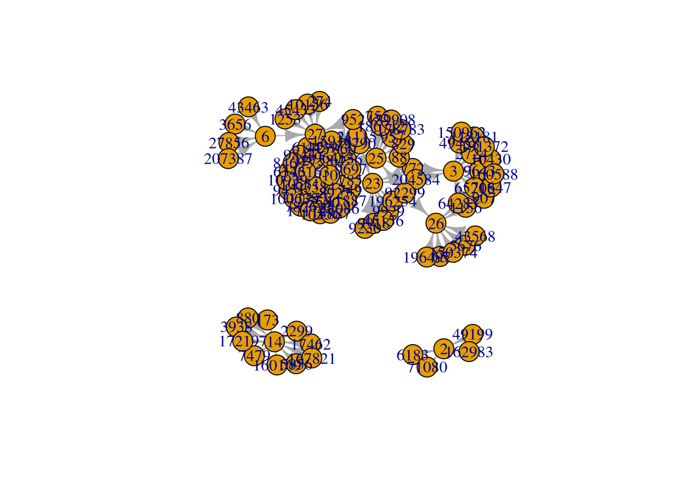

A tk application can launched to show the plot interactively:

plot(g, layout = layout.fruchterman.reingold)

Some metrics:

metrics <- data.frame(
  deg = degree(g),
  bet = betweenness(g),
  clo = closeness(g),
  eig = evcent(g)$vector,
  cor = graph.coreness(g)
)

Warning: `evcent()` was deprecated in igraph 2.0.0.
ℹ Please use `eigen_centrality()` instead.

Warning: `graph.coreness()` was deprecated in igraph 2.0.0.
ℹ Please use `coreness()` instead.

#
head(metrics)

       deg bet       clo          eig cor
6183     1   0 1.0000000 5.672735e-17   1
49199    1   0 1.0000000 5.157032e-17   1
71080    1   0 1.0000000 5.672735e-17   1
162983   1   0 1.0000000 4.641329e-17   1
772      3   0 0.3333333 1.040854e-01   2
907      1   0 1.0000000 8.141832e-03   1

The metrics above can be interpreted as follows:

• degree: local connectivity of each node
• betweenness: how frequently a node lies on shortest paths
• closeness: how quickly a node can reach other nodes
• eig: influence based on connections to influential nodes
• cor: core-periphery position in the network

For better graph readability, filter to the largest connected component or top nodes by degree before plotting labels.

library(ggplot2)

ggplot(
  metrics,
  aes(x=bet, y=eig,
    label=rownames(metrics),
    colour=res, size=abs(res))
)+
xlab("Betweenness Centrality")+
ylab("Eigenvector Centrality")+
geom_text()
+
theme(title="Key Actor Analysis")


V(g)$label.cex <- 2.2 * V(g)$degree / max(V(g)$degree)+ .2
V(g)$label.color <- rgb(0, 0, .2, .8)
V(g)$frame.color <- NA
egam <- (log(E(g)$weight)+.4) / max(log(E(g)$weight)+.4)
E(g)$color <- rgb(.5, .5, 0, egam)
E(g)$width <- egam
# plot the graph in layout1
plot(g, layout=layout1)

Further information:

http://sna.stanford.edu/lab.php?l=1