Chapter 5 Evaluation of Models
Once we obtain the model with the training data, we need to evaluate it with some new data (testing data).
No Free Lunch theorem In the absence of any knowledge about the prediction problem, no model can be said to be uniformly better than any other
5.1 Building and Validating a Model
We cannot use the the same data for training and testing (it is like evaluating a student with the exercises previously solved in class, the student’s marks will be “optimistic” and we do not know about student capability to generalise the learned concepts).
Therefore, we should, at a minimum, divide the dataset into training and testing, learn the model with the training data and test it with the rest of data as explained next.
5.1.1 Holdout approach
Holdout approach consists of dividing the dataset into training (typically approx. 2/3 of the data) and testing (approx 1/3 of the data). + Problems: Data can be skewed, missing classes, etc. if randomly divided. Stratification ensures that each class is represented with approximately equal proportions (e.g., if data contains approximately 45% of positive cases, the training and testing datasets should maintain similar proportion of positive cases).
Holdout estimate can be made more reliable by repeating the process with different subsamples (repeated holdout method).
The error rates on the different iterations are averaged (overall error rate).
- Usually, part of the data points are used for building the model and the remaining points are used for validating the model. There are several approaches to this process.
- Validation Set approach: it is the simplest method. It consists of randomly dividing the available set of observations into two parts, a training set and a validation set or hold-out set. Usually 2/3 of the data points are used for training and 1/3 is used for testing purposes.

Hold out validation
5.1.2 Cross Validation (CV)
k-fold Cross-Validation involves randomly dividing the set of observations into \(k\) groups, or folds, of approximately equal size. One fold is treated as a validation set and the method is trained on the remaining \(k-1\) folds. This procedure is repeated \(k\) times. If \(k\) is equal to \(n\) we are in the previous method.
1st step: split dataset (\(\cal D\)) into \(k\) subsets of approximately equal size \(C_1, \dots, C_k\)
2nd step: we construct a dataset \(D_i = D-C_i\) used for training and test the accuracy of the classifier \(D_i\) on \(C_i\) subset for testing
Having done this for all \(k\) we estimate the accuracy of the method by averaging the accuracy over the \(k\) cross-validation trials
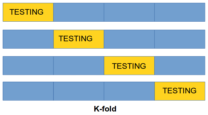
k-fold
5.1.3 Leave-One-Out Cross-Validation (LOO-CV)
- Leave-One-Out Cross-Validation (LOO-CV): This is a special case of CV. Instead of creating two subsets for training and testing, a single observation is used for the validation set, and the remaining observations make up the training set. This approach is repeated \(n\) times (the total number of observations) and the estimate for the test mean squared error is the average of the \(n\) test estimates.
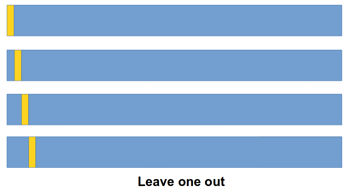
Leave One Out
5.2 Evaluation of Classification Models
The confusion matrix (which can be extended to multiclass problems) is a table that presents the results of a classification algorithm. The following table shows the possible outcomes for binary classification problems:
| \(Act Pos\) | \(Act Neg\) | |
|---|---|---|
| \(Pred Pos\) | \(TP\) | \(FP\) |
| \(Pred Neg\) | \(FN\) | \(TN\) |
where True Positives (\(TP\)) and True Negatives (\(TN\)) are respectively the number of positive and negative instances correctly classified, False Positives (\(FP\)) is the number of negative instances misclassified as positive (also called Type I errors), and False Negatives (\(FN\)) is the number of positive instances misclassified as negative (Type II errors).
From the confusion matrix, we can calculate:
True positive rate, or recall (\(TP_r = recall = TP/TP+FN\)) is the proportion of positive cases correctly classified as belonging to the positive class.
False negative rate (\(FN_r=FN/TP+FN\)) is the proportion of positive cases misclassified as belonging to the negative class.
False positive rate (\(FP_r=FP/FP+TN\)) is the proportion of negative cases misclassified as belonging to the positive class.
True negative rate (\(TN_r=TN/FP+TN\)) is the proportion of negative cases correctly classified as belonging to the negative class.
There is a trade-off between \(FP_r\) and \(FN_r\) as the objective is minimize both metrics (or conversely, maximize the true negative and positive rates). It is possible to combine both metrics into a single figure, predictive \(accuracy\):
\[accuracy = \frac{TP + TN}{TP + TN + FP + FN}\]
to measure performance of classifiers (or the complementary value, the error rate which is defined as \(1-accuracy\))
Precision, fraction of relevant instances among the retrieved instances, \[\frac{TP}{TP+FP}\]
Recall$ (\(sensitivity\) probability of detection, \(PD\)) is the fraction of relevant instances that have been retrieved over total relevant instances, \(\frac{TP}{TP+FN}\)
f-measure is the harmonic mean of precision and recall, \(2 \cdot \frac{precision \cdot recall}{precision + recall}\)
G-mean: \(\sqrt{PD \times Precision}\)
G-mean2: \(\sqrt{PD \times Specificity}\)
J coefficient, \(j-coeff = sensitivity + specificity - 1 = PD-PF\)
A suitable and interesting performance metric for binary classification when data are imbalanced is the Matthew’s Correlation Coefficient (\(MCC\))~:
\[MCC=\frac{TP\times TN - FP\times FN}{\sqrt{(TP+FP)(TP+FN)(TN+FP)(TN+FN)}}\]
\(MCC\) can also be calculated from the confusion matrix. Its range goes from -1 to +1; the closer to one the better as it indicates perfect prediction whereas a value of 0 means that classification is not better than random prediction and negative values mean that predictions are worst than random.
5.2.1 Prediction in probabilistic classifiers
A probabilistic classifier estimates the probability of each of the posible class values given the attribute values of the instance \(P(c|{x})\). Then, given a new instance, \({x}\), the class value with the highest a posteriori probability will be assigned to that new instance (the winner takes all approach):
\(\psi({x}) = argmax_c (P(c|{x}))\)
5.3 Other Metrics used in Software Engineering with Classification
In the domain of defect prediction and when two classes are considered, it is also customary to refer to the probability of detection, (\(pd\)) which corresponds to the True Positive rate (\(TP_{rate}\) or ) as a measure of the goodness of the model, and probability of false alarm (\(pf\)) as performance measures~.
The objective is to find which techniques that maximise \(pd\) and minimise \(pf\). As stated by Menzies et al., the balance between these two measures depends on the project characteristics (e.g. real-time systems vs. information management systems) it is formulated as the Euclidean distance from the sweet spot \(pf=0\) and \(pd=1\) to a pair of \((pf,pd)\).
\[balance=1-\frac{\sqrt{(0-pf^2)+(1-pd^2)}}{\sqrt{2}}\]
It is normalized by the maximum possible distance across the ROC square (\(\sqrt{2}, 2\)), subtracted this value from 1, and expressed it as a percentage.
5.4 Graphical Evaluation
5.4.1 Receiver Operating Characteristic (ROC)
The Receiver Operating Characteristic (\(ROC\))(Fawcett 2006) curve which provides a graphical visualisation of the results.
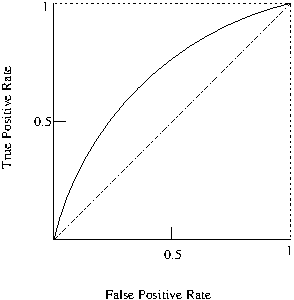
Receiver Operating Characteristic
The Area Under the ROC Curve (AUC) also provides a quality measure between positive and negative rates with a single value.
A simple way to approximate the AUC is with the following equation: \(AUC=\frac{1+TP_{r}-FP_{r}}{2}\)
5.4.2 Precision-Recall Curve (PRC)
Similarly to ROC, another widely used evaluation technique is the Precision-Recall Curve (PRC), which depicts a trade off between precision and recall and can also be summarised into a single value as the Area Under the Precision-Recall Curve (AUPRC)~.
%AUPCR is more accurate than the ROC for testing performances when dealing with imbalanced datasets as well as optimising ROC values does not necessarily optimises AUPR values, i.e., a good classifier in AUC space may not be so good in PRC space. %The weighted average uses weights proportional to class frequencies in the data. %The weighted average is computed by weighting the measure of class (TP rate, precision, recall …) by the proportion of instances there are in that class. Computing the average can be sometimes be misleading. For instance, if class 1 has 100 instances and you achieve a recall of 30%, and class 2 has 1 instance and you achieve recall of 100% (you predicted the only instance correctly), then when taking the average (65%) you will inflate the recall score because of the one instance you predicted correctly. Taking the weighted average will give you 30.7%, which is much more realistic measure of the performance of the classifier.
5.5 Numeric Prediction Evaluation
In the case of defect prediction, it matters the difference between the predicted value and the actual value. Common performance metrics used for numeric prediction are as follows, where \(\hat{y_n}\) represents the predicted value and \(y_n\) the actual one.
Mean Square Error (\(MSE\))
\(MSE = \frac{(\hat{y_1} - y_1)^2 + \ldots +(\hat{y_n} - y_n)^2}{n} = \frac{1}{n}\sum_{i=1}^n(\hat{y_i} - y_i)^2\)
Root mean-squared error (\(RMSE\))
\({RMSE} = \sqrt{\frac{\sum_{t=1}^n (\hat y_t - y)^2}{n}}\)
Mean Absolute Error (\(MAE\))
\(MAE = \frac{|\hat{y_1} - y_1| + \ldots +|\hat{y_n} - y_n|}{n} = \sqrt{\frac{\sum_{t=1}^n |\hat y_t - y|}{n}}\)
Relative Absolute Error (\(RAE\))
\(RAE = \frac{ \sum^N_{i=1} | \hat{\theta}_i - \theta_i | } { \sum^N_{i=1} | \overline{\theta} - \theta_i |}\)
Root Relative-Squared Error (\(RRSE\))
\(RRSE = \sqrt{ \frac{ \sum^N_{i=1} | \hat{\theta}_i - \theta_i | } { \sum^N_{i=1} | \overline{\theta} - \theta_i | } }\)
where \(\hat{\theta}\) is a mean value of \(\theta\).
Relative-Squared r (\(RSE\))
\(\frac{(p_1-a_1)^2 + \ldots +(p_n-a_n)^2}{(a_1-\hat{a})^2 + \ldots + (a_n-\hat{a})^2}\)
where (\(\hat{a}\) is the mean value over the training data)
Relative Absolute Error (\(RAE\))
Correlation Coefficient
Correlation coefficient between two random variables \(X\) and \(Y\) is defined as \(\rho(X,Y) = \frac{{\bf Cov}(X,Y)}{\sqrt{{\bf Var}(X){\bf Var}(Y)}}\). The sample correlation coefficient} \(r\) between two samples \(x_i\) and \(y_j\) is vvdefined as \(r = S_{xy}/\sqrt{S_{xx}S_{yy}}\)
Example: Is there any linear relationship between the effort estimates (\(p_i\)) and actual effort (\(a_i\))?
\(a\|39,43,21,64,57,47,28,75,34,52\)
\(p\|65,78,52,82,92,89,73,98,56,75\)
p<-c(39,43,21,64,57,47,28,75,34,52)
a<-c(65,78,52,82,92,89,73,98,56,75)
#
cor(p,a)
## [1] 0.84\(R^2\)