Chapter 11 Text Mining Software Engineering Data
In software engineering, there is a lot of information in plain text such as requirements, bug reports, mails, reviews from applicatons, etc. Typically that information can be extracted from Software Configuration Management Systems (SCM), Bug Tracking Systems (BTS) such as Bugzilla or application stores such as Google Play or Apple’s AppStore, etc. can be mined to extract relevant information. Here we briefly explain the text mining process and how this can be done with R.
A well-known package for text mining is tm Feinerer, Hornik, and Meyer (2008). Another popular package is wordcloud.
11.1 Terminology
The workflow that we follow for analyzing a set of text documents are:
- Importing data. A Corpus is a collection of text documents, implemented as VCorpus (corpora are R object held in memory). The
tmprovides several corpus constructors:DirSource,VectorSource, orDataframeSource(getSources()).
There are several parameters that control the creation of a Corpus. ((The parameter readerControl of the corpus constructor has to be a list with the named components reader and language))
Preprocessing: in this step we may remove common words, punctuation and we may perform other operations. We may do this operations after creating the DocumentTermMatrix.
Inspecting and exploring data: Individual documents can be accessed via [[
Transformations: Transformations are done via the
tm_map()function. +tm_map(_____, stripWhitespace)
+tm_map(_____, content_transformer(tolower))+tm_map(_____, removeWords, stopwords("english"))+tm_map(_____, stemDocument)Creating
Term-DocumentMatrices: TermDocumentMatrix and DocumentTermMatrix + A document term matrix is a matrix with documents as the rows and terms as the columns. Each cell of the matrix contains the count of the frequency of words. We use DocumentTermMatrix() to create the matrix. +inspect(DocumentTermMatrix( newsreuters, list(dictionary = c("term1", "term2", "term3")))). It displays detailed information on a corpus or a term-document matrix.Relationships between terms. +
findFreqTerms(_____, anumber)+findAssocs(Mydtm, "aterm", anumbercorrelation)+ A dictionary is a (multi-)set of strings. It is often used to denote relevant terms in text mining.Clustering and Classification
11.2 Example of classifying bugs from Bugzilla
Bugzilla is Issue Tracking System that allow us to follow the evolution of a project.
The following example shows how to work with entries from Bugzilla. It is assumed that the data has been extracted and we have the records in a flat file (this can be done using Web crawlers or directly using the SQL database).
library(foreign)
# path_name <- file.path("C:", "datasets", "textMining")
# path_name
# dir(path_name)

#Import data
options(stringsAsFactors = FALSE)
d <- read.arff("./datasets/textMining/reviewsBugs.arff" )
str(d) #print out information about d
## 'data.frame': 789 obs. of 2 variables:
## $ revContent: chr "Can't see traffic colors now With latest updates I can't see the traffic green/red/yellow - I have to pull over"| __truncated__ "Google Map I like it so far, it has not steered me wrong." "Could be 100X better Google should start listening to customers then they'd actually build a proper product." "I like that! Easily more helpful than the map app that comes with your phone." ...
## $ revBug : Factor w/ 2 levels "N","Y": 2 1 1 1 1 1 2 1 2 1 ...head(d,2) # the first two rows of d. ## revContent
## 1 Can't see traffic colors now With latest updates I can't see the traffic green/red/yellow - I have to pull over and zoom in the map so that one road fills the entire screen. Traffic checks are (were) the only reason I use google maps!
## 2 Google Map I like it so far, it has not steered me wrong.
## revBug
## 1 Y
## 2 N# fifth entry
d$revContent[5]## [1] "Just deleted No I don't want to sign in or sign up for anything stop asking"d$revBug[5]## [1] N
## Levels: N YCreating a Document-Term Matrix (DTM)
Now, we can explore things such as “which words are associated with”feature”?”
# which words are associated with "bug"?
findAssocs(dtm, 'bug', .3) # minimum correlation of 0.3. Change accordingly.
## $bug
## it? mini major users causing ipad
## 1.00 0.92 0.91 0.80 0.62 0.57And find frequent terms.
findFreqTerms(dtm, 15) #terms that appear 15 or more times, in this case## [1] "google" "map" "like" "app" "just" "good"
## [7] "crashes" "maps" "time" "get" "much" "really"
## [13] "update" "great" "nice" "best" "ever" "fun"
## [19] "review" "love" "awesome" "cool" "amazing" "game"
## [25] "clans" "clash" "game." "game!" "addicting" "play"
## [31] "playing" "addictive"Remove some terms
sparseparam <- 0.90 # will make the matrix 90% empty space, maximum. Change this, as you like.
dtm_sprs <- removeSparseTerms(dtm,sparse=sparseparam)
inspect(dtm_sprs)
## <<DocumentTermMatrix (documents: 789, terms: 9)>>
## Non-/sparse entries: 1233/5868
## Sparsity : 83%
## Maximal term length: 7
## Weighting : term frequency - inverse document frequency (normalized) (tf-idf)
## Sample :
## Terms
## Docs app awesome best clash fun game good great love
## 159 0 0.00 0 1.6 0 0 0.0 0 1.46
## 163 0 3.12 0 0.0 0 0 0.0 0 0.00
## 178 0 3.12 0 0.0 0 0 0.0 0 0.00
## 400 0 0.00 0 0.0 0 0 3.1 0 0.00
## 421 0 0.00 0 0.0 0 0 3.1 0 0.00
## 472 0 0.00 0 0.0 0 0 3.1 0 0.00
## 50 0 0.00 0 0.0 0 0 3.1 0 0.00
## 525 0 1.56 0 0.0 0 0 0.0 0 1.46
## 527 0 0.00 0 0.0 0 0 3.1 0 0.00
## 532 0 0.00 0 1.6 0 0 0.0 0 1.46maintitle <-paste0("Most frequent terms (sparseness=" ,sparseparam , " )")
barplot(as.matrix(dtm_sprs),xlab="terms",ylab="number of occurrences", main=maintitle)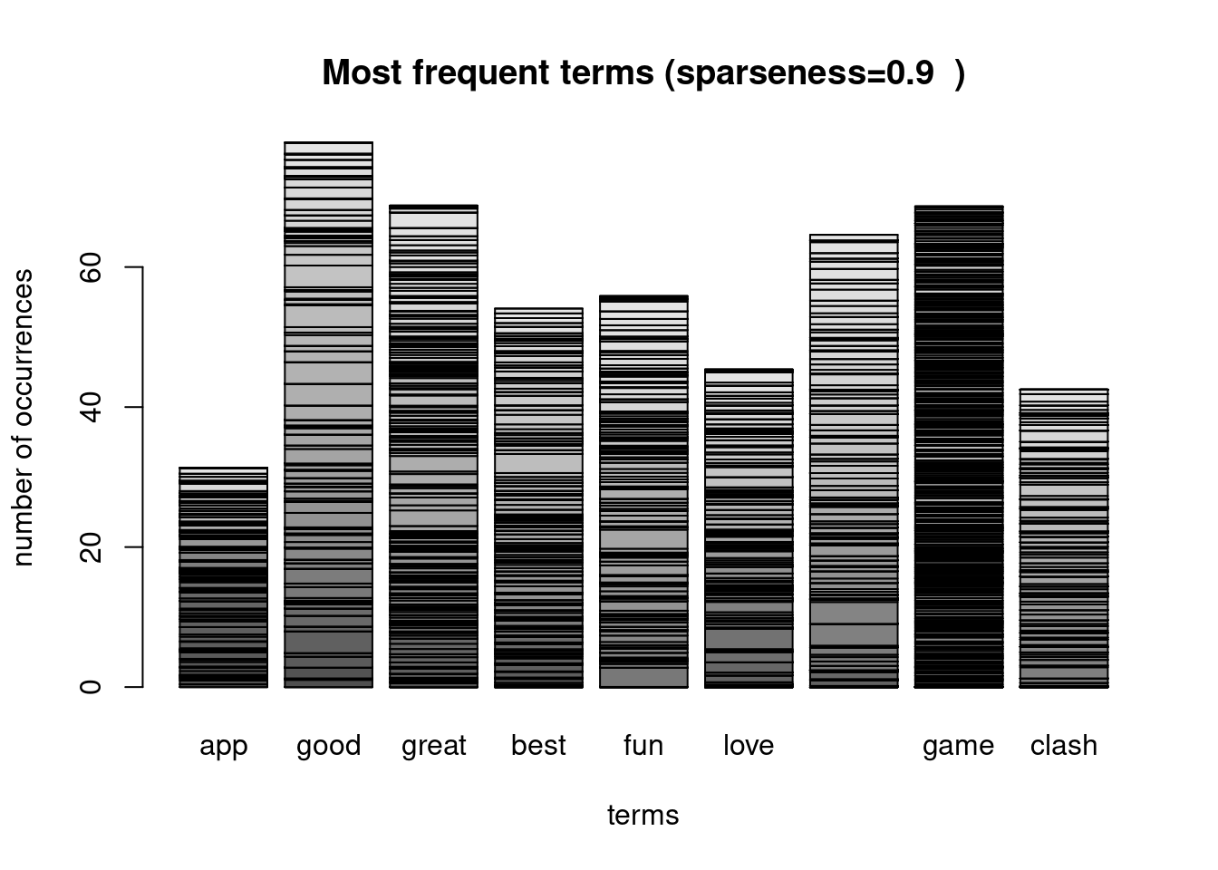
# organize terms by their frequency

freq_dtm_sprs <- colSums(as.matrix(dtm_sprs))
length(freq_dtm_sprs)
## [1] 9sorted_freq_dtm_sprs <- sort(freq_dtm_sprs, decreasing = TRUE)
sorted_freq_dtm_sprs## good great game awesome fun best love clash app
## 77.8 68.8 68.7 64.6 55.8 54.1 45.4 42.5 31.3Create a data frame that will be the input to the classifier. Last column will be the label.
As data frame:
#dtmdf <- as.data.frame(dtm.90)
#dtmdf <- as.data.frame(inspect(dtm_sprs))
dtmdf <- as.data.frame(as.matrix(dtm_sprs))
# rownames(dtm)<- 1:nrow(dtm)

class <- d$revBug
dtmdf <- cbind(dtmdf,class)
head(dtmdf, 3)
Use any classifier now: - split the dataframe into training and testing - Build the classification model using the training subset - apply the model to the testing subset and obtain the Confusion Matrix - Analise the results
library(caret)
library(randomForest)


inTraining <- createDataPartition(dtmdf$class, p = .75, list = FALSE)
training <- dtmdf[ inTraining,]
testing  <- dtmdf[-inTraining,]

fitControl <- trainControl(## 5-fold CV
                           method = "repeatedcv",
                           number = 5,
                           ## repeated ten times
                           repeats = 5)


gbmFit1 <- train(class ~ ., data = training,
                 method = "gbm",
                 trControl = fitControl,
                 ## This last option is actually one
                 ## for gbm() that passes through
                 verbose = FALSE)

gbmFit1
## Stochastic Gradient Boosting
##
## 593 samples
## 9 predictor
## 2 classes: 'N', 'Y'
##
## No pre-processing
## Resampling: Cross-Validated (5 fold, repeated 5 times)
## Summary of sample sizes: 475, 474, 474, 474, 475, 475, ...
## Resampling results across tuning parameters:
##
## interaction.depth n.trees Accuracy Kappa
## 1 50 0.798 0.000
## 1 100 0.801 0.081
## 1 150 0.806 0.189
## 2 50 0.805 0.149
## 2 100 0.802 0.219
## 2 150 0.798 0.211
## 3 50 0.806 0.215
## 3 100 0.802 0.236
## 3 150 0.801 0.233
##
## Tuning parameter 'shrinkage' was held constant at a value of 0.1
##
## Tuning parameter 'n.minobsinnode' was held constant at a value of 10
## Accuracy was used to select the optimal model using the largest value.
## The final values used for the model were n.trees = 50, interaction.depth =
## 3, shrinkage = 0.1 and n.minobsinnode = 10.# trellis.par.set(caretTheme())
# plot(gbmFit1)
#
# trellis.par.set(caretTheme())
# plot(gbmFit1, metric = "Kappa")
head(predict(gbmFit1, testing, type = "prob"))## N Y
## 1 0.690 0.3105
## 2 0.583 0.4166
## 3 0.690 0.3105
## 4 0.908 0.0919
## 5 0.353 0.6472
## 6 0.690 0.3105conf_mat <- confusionMatrix(testing$class, predict(gbmFit1, testing))
conf_mat## Confusion Matrix and Statistics
##
## Reference
## Prediction N Y
## N 152 5
## Y 27 12
##
## Accuracy : 0.837
## 95% CI : (0.777, 0.886)
## No Information Rate : 0.913
## P-Value [Acc > NIR] : 0.999819
##
## Kappa : 0.35
##
## Mcnemar's Test P-Value : 0.000205
##
## Sensitivity : 0.849
## Specificity : 0.706
## Pos Pred Value : 0.968
## Neg Pred Value : 0.308
## Prevalence : 0.913
## Detection Rate : 0.776
## Detection Prevalence : 0.801
## Balanced Accuracy : 0.778
##
## 'Positive' Class : N
## We may compute manually all derived variables from the Confusion Matrix. See Section – with the description of the Confusion Matrix
# str(conf_mat)
TruePositive <- conf_mat$table[1,1]
TruePositive
## [1] 152FalsePositive <- conf_mat$table[1,2]
FalsePositive## [1] 5FalseNegative <- conf_mat$table[2,1]
FalseNegative## [1] 27TrueNegative <- conf_mat$table[2,2]
TrueNegative## [1] 12# Sum columns in the confusion matrix
ConditionPositive <- TruePositive + FalseNegative
ConditionNegative <- FalsePositive + TrueNegative
TotalPopulation <- ConditionPositive + ConditionNegative
TotalPopulation## [1] 196#Sum rows in the confusion matrix
PredictedPositive <- TruePositive + FalsePositive
PredictedNegative <- FalseNegative + TrueNegative
# Total Predicted must be equal to the total population
PredictedPositive+PredictedNegative## [1] 196SensitivityRecall_TPR <- TruePositive / ConditionPositive
SensitivityRecall_TPR## [1] 0.849Specificity_TNR_SPC <- TrueNegative / ConditionNegative
Specificity_TNR_SPC## [1] 0.706Precision_PPV <- TruePositive / PredictedPositive
Precision_PPV ## [1] 0.968NegativePredictedValue_NPV <- TrueNegative / PredictedNegative
NegativePredictedValue_NPV## [1] 0.308Prevalence <- ConditionPositive / TotalPopulation
Prevalence## [1] 0.913Accuracy_ACC <- (TruePositive + TrueNegative) / TotalPopulation
Accuracy_ACC## [1] 0.837FalseDiscoveryRate_FDR <- FalsePositive / PredictedPositive
FalseDiscoveryRate_FDR## [1] 0.0318FalseOmisionRate_FOR <- FalseNegative / PredictedNegative
FalseOmisionRate_FOR## [1] 0.692FallOut_FPR <- FalsePositive / ConditionNegative
FallOut_FPR## [1] 0.294MissRate_FNR <- FalseNegative / ConditionPositive
MissRate_FNR ## [1] 0.151And finally, a word cloud as an example that appears everywhere these days.
library(wordcloud)

# calculate the frequency of words and sort in descending order.
wordFreqs=sort(colSums(as.matrix(dtm_sprs)),decreasing=TRUE)

wordcloud(words=names(wordFreqs),freq=wordFreqs)
11.3 Extracting data from Twitter
The hardest bit is to link with Twitter. Using the TwitteR package is explained following this example.