Chapter 12 Time Series
Many sources of information are time related. For example, data from Software Configuration Management (SCM) such as Git, GitHub) systems or Dashboards such as Metrics Grimoire from Bitergia or SonarQube
With MetricsGrimore or SonarQube we can extract datasets or dump of databases. For example, a dashboard for the OpenStack project is located at http://activity.openstack.org/dash/browser/ and provides datasets as MySQL dumps or JSON files.
With R we can read a JSON file as follows:
library(jsonlite)
# Get the JSON data
# gm <- fromJSON("http://activity.openstack.org/dash/browser/data/json/nova.git-scm-rep-evolutionary.json")
gm <- fromJSON('./datasets/timeSeries/nova.git-scm-rep-evolutionary.json')
str(gm)
## List of 13
## $ added_lines : num [1:287] 431874 406 577 697 7283 ...
## $ authors : int [1:287] 1 1 4 2 7 5 4 9 8 11 ...
## $ branches : int [1:287] 1 1 1 1 1 1 1 1 1 1 ...
## $ commits : int [1:287] 3 4 16 11 121 38 35 90 66 97 ...
## $ committers : int [1:287] 1 1 4 2 7 5 4 9 8 11 ...
## $ date : chr [1:287] "May 2010" "May 2010" "Jun 2010" "Jun 2010" ...
## $ files : int [1:287] 1878 9 13 7 144 111 28 1900 89 101 ...
## $ id : int [1:287] 0 1 2 3 4 5 6 7 8 9 ...
## $ newauthors : int [1:287] 1 1 2 0 4 1 0 4 2 3 ...
## $ removed_lines: num [1:287] 864 530 187 326 2619 ...
## $ repositories : int [1:287] 1 1 1 1 1 1 1 1 1 1 ...
## $ unixtime : chr [1:287] "1274659200" "1275264000" "1275868800" "1276473600" ...
## $ week : int [1:287] 201021 201022 201023 201024 201025 201026 201027 201028 201029 201030 ...Now we can use time series packages. First, after loading the libraries, we need to create a time series object.
# TS libraries
library(xts)
##
## Attaching package: 'xts'## The following objects are masked from 'package:dplyr':
##
## first, lastlibrary(forecast)
# Library to deal with dates
library(lubridate)
# Ceate a time series object
gmts <- xts(gm$commits,seq(ymd('2010-05-22'),ymd('2015-11-16'), by = '1 week'))
# TS Object
str(gmts)## An 'xts' object on 2010-05-22/2015-11-14 containing:
## Data: int [1:287, 1] 3 4 16 11 121 38 35 90 66 97 ...
## Indexed by objects of class: [Date] TZ: UTC
## xts Attributes:
## NULLhead(gmts, 3)## [,1]
## 2010-05-22 3
## 2010-05-29 4
## 2010-06-05 16Visualise the time series object
plot(gmts)
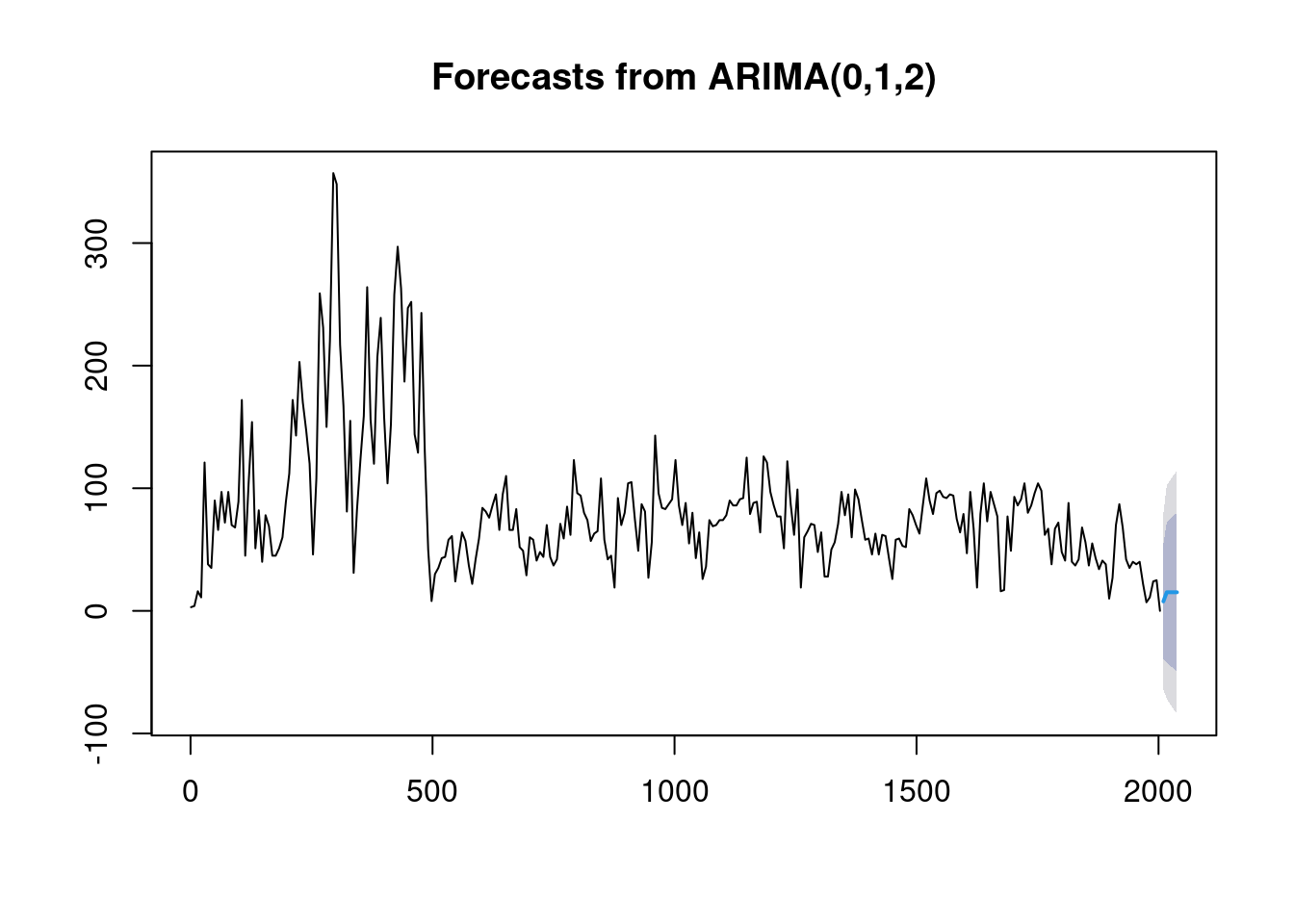
Arima model:
fit <- auto.arima(gmts)
fit
## Series: gmts
## ARIMA(0,1,2)
##
## Coefficients:
## ma1 ma2
## -0.312 -0.307
## s.e. 0.058 0.064
##
## sigma^2 = 1341: log likelihood = -1435
## AIC=2876 AICc=2876 BIC=2887forecast(fit, 5)## Point Forecast Lo 80 Hi 80 Lo 95 Hi 95
## 2010 7.75 -39.2 54.7 -64.0 79.5
## 2017 15.16 -41.8 72.1 -72.0 102.3
## 2024 15.16 -44.6 74.9 -76.2 106.5
## 2031 15.16 -47.2 77.5 -80.2 110.5
## 2038 15.16 -49.7 80.0 -84.0 114.3plot(forecast(fit, 5))